How Much Does It Cost to Train a Large Language Model? A Guide

Machine learning is affecting every sector, and no one seems to have a clear idea about how much it costs to train a specialized LLM. This week at OpenAI Dev Day 2023, the company announced their model-building service for $2-3M minimum. This is a steep price to pay for a specialized model, and many are wondering, is it necessary?

The question of how much it costs to train an LLM is a really hard one, and while there’s not a straightforward, plug-and-chug cost calculation, the answer mainly depends on two factors: compute requirements and how long it takes to train.

To help provide clarity on how to estimate the cost of training an LLM, I’ve compiled a structured overview of the different levers that affect model training time and compute requirements.

Note that this article does not include costs of:

• Development and operation (eng salaries, debugging, IDEs, version control systems, tooling to monitor model performance, infrastructure set-up (try Brev lol)
• Using more optimized ML libraries / APIs (decreasing cost)
• Code licensing / legal considerations
• Data privacy/security & regulatory compliance
• Model bias & fairness assessments / ethical reviews
• Adversarial training (to protect against adversarial attacks) & other security measures
• Deployment in a production environment

The three main variables to consider when determining compute requirements and training time are model architecture, training dynamics, and methods for optimizing training performance. First, however, we should learn a bit about the hardware these models fit on, so we understand the context of where these variables fit.

Hardware Costs

This refers to access to GPUs and their associated cost, and GPU memory tends to the bottleneck. This is how much “stuff” (model, parameters, etc.) the GPU is able to hold in memory at one time. Something we’ve noticed is that most people think they need an expensive, highly elusive A100 or H100 with 40GB or 80GB of GPU memory. However, something smaller, cheaper, and more available may suffice.

I’ve released a few guides on fine-tuning (Mistral on HF dataset, Mistral on own dataset, Llama on own dataset). In these guides, I used QLoRA with 4-bit quantization and LoRA on all linear layers, reducing the trainable parameters by 98%. As a result, I was able to train these models on a single A10G (24GB of GPU Memory, and only $1/hr on Brev, which provides cloud GPUs without vendor lock-in across cloud providers, like AWS, GCP, and Lambda Labs). Training on my own dataset took about 10 minutes for 500 iterations over 200 samples, and training on the HF dataset took about an hour for 6,000 samples and 1000 iterations. These models would likely not be production-grade; I am just providing these values as base references.

Cloud provider costs and the choice between spot and reserved instances are direct cost factors. If using cloud GPUs, different providers and regions can have vastly different pricing. Spot instances are cheaper but less reliable as you may lose them while training, while reserved instances cost more but ensure availability.

Model Architecture

Size and Structure

The depth (number of layers), width (neurons per layer), and the total number of parameters affect both GPU memory requirements and training time. A model with more and/or wider layers has the capacity to learn more complex features, but at the expense of increased computational demand. Increasing the total number of parameters to train increases the estimated time to train and the GPU memory requirements. Techniques like low-rank matrix factorization (e.g., LoRA and sparsity, where tensors are pruned to have a high number of 0 values, can reduce the number of trainable parameters and mitigate these costs, but they require careful tuning. Sparsity is often done in transformer attention mechanisms (see below) or in weights (as in block-sparse models).

Attention Mechanisms

Transformers leverage self-attention mechanisms, with multiple heads attending to different sequence parts, enhancing learning at the cost of increased computation. The traditional Transformer attention style compares every token in the context window with every other token, leading to memory requirements that are quadratic in the size of the context window, $O(n^2)$. Sparse attention models offer a compromise by focusing on a subset of positions, for example with local (nearby) attention, thereby reducing computational load, often down to $O(n \sqrt{n})$ (source).

Efficiency Optimizations

Choices of activation functions and gating mechanisms can impact computational intensity and training time. Different activation functions have varying levels of mathematical complexity; ReLU, for example, is less complex than sigmoid or tanh. Additionally, parameter sharing, for example weight sharing across layers, can reduce the number of unique parameters and hence memory requirements.

Training Dynamics

Learning Rate and Batch Size

Learning rate and batch size significantly influence the model's training speed and stability. The learning rate of a model affects the step size it takes in the opposite direction of the gradient (i.e. the direction towards minimizing the cost or loss function). This is called gradient descent. The batch size is the number of samples processed before the model’s parameters are updated. It is true that the larger your batch, the more memory you need; it scales linearly with the size of the batch. However, a larger batch size can lead to faster convergence because at each step, you get better estimates of the true gradient.

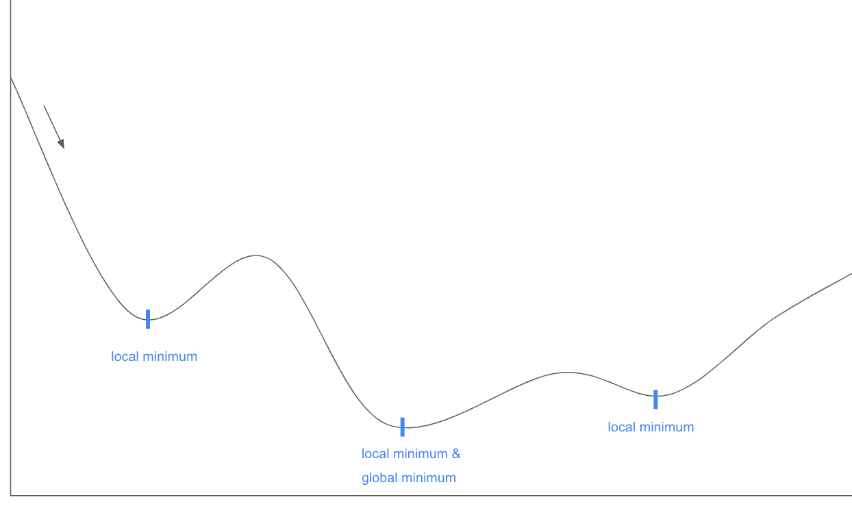
One subtlety to consider: Even if you had a terabyte of GPU memory, you still may not want to use the largest batch size possible. Downsampling (i.e. using a smaller batch size than the total number of training samples) introduces noise into the gradient, which can help you avoid local minima. That’s why it’s called stochastic gradient descent: the stochasticity refers to how much you’re downsampling from your training set in each batch.

The learning rate's size (magnitude) and schedule (rate of change over training) can affect the speed and stability of convergence. A higher learning rate means the model takes bigger steps during gradient descent. While this can speed up convergence, it can also lead to overshooting minima and potentially unstable training. Conversely, a learning rate that is too small can slow down convergence (as getting to a minimum takes longer), and the model may get stuck in local minima. See the drawing below for an example of local vs. global minima. In simple terms, a local minimum that is not equal to the global minimum is a location on the graph where it seems like the optimal loss has been found, but we had just gone a little further - up a hill and dealing with some worse performance to get there - we could have found a better place in the graph.

Precision and Quantization

The precision of calculations, like FP16 versus FP32 - using 16 bits to represent each floating point versus 32 - and techniques such as quantization balance memory usage with performance trade-offs. Using half-precision (FP16) instead of single-precision (FP32) floating points cuts the tensor sizes in half, which can save memory and speed up training by enabling faster operations and more parallelization. However, this comes with a trade-off in precision, which can lead to potential numerical errors, like overflow/underflow errors, as fewer bits can’t represent as large or as small numbers. It can also reduce accuracy, but if not too extreme, it can serve as a form of regularization, reducing overfitting and allowing the model to actually perform better on the held-out dataset. Another technique is to use mixed precision training, where some floating points are FP16 and some are FP32. Determining which matrices should be represented as FP16 vs. FP32 may take some experimentation, however, which is also a cost consideration.

Quantization is another technique that maps high-precision floating points to lower-precision values, usually 8- or even 4-bit fixed-point representation integers. This reduces tensor sizes by 75% or even 87.5%, but usually results in a significant reduction in model accuracy; as mentioned before, though, it may actually help the model generalize better, so experimentation may be worthwhile.

Hyperparameter Sweeps

Hyperparameters are external configuration variables for machine learning models, i.e. they aren’t learned by the model itself, like weights are. Hyperparameters are basically all the variables we discussed here: learning rate, model architecture like number of neurons or layers, attention mechanisms, etc. Hyperparameter sweeps are when experiments are run training different models with combinations of various hyperparameter settings, and they enable a model to find the best possible combinations of hyperparameter values for its specific dataset and task. However, it is computationally expensive, as you must train many models to find the best configuration.

Checkpointing/Early Stopping

Frequent model state saving (checkpointing) can increase disk usage but provides more rollback points; if a model overfits or performs better at an earlier state in training, you can have those weights saved at a checkpoint and load that model. Early stopping is a method where one stops model training after it ceases to improve on the held out validations set. This can save training time.

Optimizing Training Performance

Base Model State

Starting with a pre-trained model, especially one that is trained in a task similar to the new task being trained, can significantly reduce training time. If the initial weights are closer to the optimal solution’s weights, training can be faster. Building a model from scratch - i.e. with randomized initial weight matrices or similar - takes significantly more compute and is usually not advised.

Parallelism and Distributed Training

Parallel computing is usually done with one computer that has multiple processors, which execute multiple tasks simultaneously for increased efficiency. Distributed computing involves several machines (that can be physically distant) working on divided tasks and then combining their results. Usually these two techniques are used together.

Parallelism can speed up training but adds complexity and compute requirements. There are various parallelization methods, like pipeline model parallelization, where models are split into different stages and distributed across GPUs, and data parallelization, where the dataset is divided across GPUs. Distributed training can be more efficient but requires more compute resources and adds complexity.

Data Considerations

How quickly the training data can be fed from storage into the model can affect training time. Some variables to consider:

• Where is the GPU located? Transferring your own data to cloud machines in more remote regions may take longer
• Machine I/O bandwidth affects time to transfer between storage and GPU
• Data caching, pre-fetching, and parallel loading on the GPU can decrease this time

Additionally, more complex data might take the model longer to learn the patterns, i.e. loss convergence time may increase.

The relevance and quality of training data also have a profound effect on training efficiency. Preprocessing and augmentation can improve outcomes but may increase the computational overhead.

Conclusion

I hope this helps to understand the complexities behind calculating how much it costs to fine-tune or train an LLM. There’s no one-size-fits-all answer or plug-and-chug equation; the main takeaway I’d like you to have is that there’s a lot of experimentation to find what works best for you and your use case, but that’s part of the fun of ML. So try things, expect a lot of it to not work, but by doing so, you’ll see what gets you the best results.

Ultimately, the cost of training LLMs like those offered by OpenAI does seem steep. For many, fine-tuning smaller models and maintaining control over proprietary data might be a more viable solution.